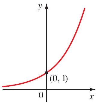
 \(f(x)=a^{x}\) for \(a>1\)
The exponential function \(f\) with base \(a\) (where \(a>0, a \neq 1\) ) is defined for all real numbers \(x\) by
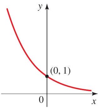
The domain of \(f\) is \(\mathbb{R}\), and the range of \(f\) is \((0, \infty)\) The graph of \(f\) has one of the following shapes, depending on the value of \(a\) :
 \(f(x)=a^{x}\) for \(a>1\)
 \(f(x)=a^{x}\) for \(0<a<1\)
The natural exponential function is the exponential function with base \(e\) :
The number \(e\) is defined to be the number that the expression \((1+1 / n)^{n}\) approaches as \(n \rightarrow \infty\). An approximate value for the irrational number \(e\) is
If a principal \(P\) is invested in an account paying an annual interest rate \(r\), compounded \(n\) times a year, then after \(t\) years the amount \(A(t)\) in the account is
If the interest is compounded continuously, then the amount is
The logarithmic function \(\log _{a}\) with base \(a\) (where \(a>0, a \neq 1\) ) is defined for \(x>0\) by
So \(\log _{a} x\) is the exponent to which the base \(a\) must be raised to give \(y\).
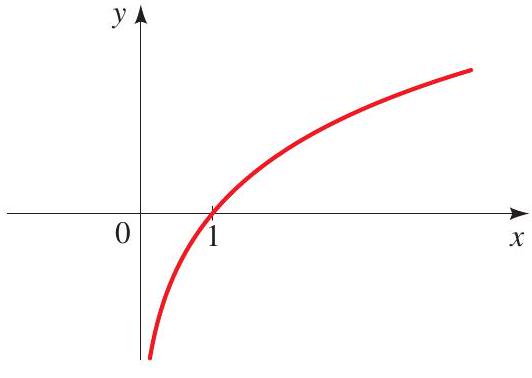
The domain of \(\log _{a}\) is \((0, \infty)\), and the range is \(\mathbb{R}\). For \(a>1\), the graph of the function \(\log _{a}\) has the following shape:

The logarithm function with base 10 is called the common logarithm and is denoted log. So
The logarithm function with base \(e\) is called the natural logarithm and is denoted \(\mathbf{l n}\). So
Let \(a\) be a logarithm base \((a>0, a \neq 1)\), and let \(A, B\), and \(C\) be any real numbers or algebraic expressions that represent real numbers, with \(A>0\) and \(B>0\). Then:
A population experiences exponential growth if it can be modeled by the exponential function
where \(n(t)\) is the population at time \(t, n_{0}\) is the initial population (at time \(t=0\) ), and \(r\) is the relative growth rate (expressed as a proportion of the population).
A population experiences logistic growth if it can be modeled by a function of the form
where \(n(t)\) is the population at time \(t, r\) is the initial relative growth rate, \(M\) is the carrying capacity of the environment, and \(A=\left(M-n_{0}\right) / n_{0}\), where \(n_{0}\) is the initial population.
If a radioactive substance with half-life \(h\) has initial mass \(m_{0}\), then at time \(t\) the mass \(m(t)\) of the substance that remains is modeled by the exponential function
where \(r=\frac{\ln 2}{h}\).
If an object has an initial temperature that is \(D_{0}\) degrees warmer than the surrounding temperature \(T_{s}\), then at time \(t\) the temperature \(T(t)\) of the object is modeled by the function
where the constant \(k>0\) depends on the size and type of the object.
The \(\mathbf{p H}\) scale measures the acidity of a solution:
The Richter scale measures the intensity of earthquakes:
The decibel scale measures the intensity of sound: